Mass Transit System Structure

The model is arranged in a hierarchy allowing the partitioning and relocation of units at different levels of the structure as described in section . This allows us to use flexible recursive algorithms to facilitate a lot of searching and reporting tasks. For example, we recursively walk the tree to produce the incremental state snapshots of the system hierarchy in graphML format for viewing in yFiles's yEd application.

Generic Cell Class

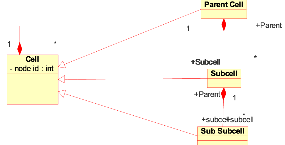
All simulation entities inherit from the Cell class, which provides a sub cell container for any children classes. The cell class stores a handle to its own parent cell as well, so algorithms may traverse the tree in either direction. Subroutines allow child cells to move about the tree, updating associations so cells never have more than one parent. Each cell also has a className to distinguish between different types of children. They also inherit filtering functions that can search for and return a list of child cells meeting certain criteria.

Figure 4.2: Cell Class Diagram

Neighborhood Nodes

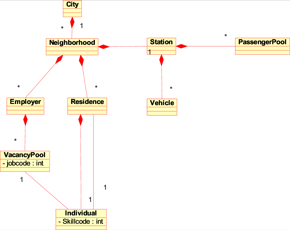
All of the elements in the model are comprised of various incarnations of the generic cell class. A master city cell forms the root of the tree hierarchy and contains several neighborhood node cells representing clusters of employers and residences that share a transit station. This hierarchy represents a realization of the general class template described in Figure 2.6. Each neighborhood can contain any number of employers or residences that share the same transit station in a pattern reminiscent of J.H Crawford's reference districts. [16]

Figure 4.3: Neighborhood Class Structure

An employer would have a number of job vacancies associated with a particular job code (representing the particular skill required of a worker) and additionally a work schedule that would dictate the employee's commute schedule. Assuming that each vacancy could draw a qualified employee into the metropolitan area, an individual would be instantiated to fill that job vacancy and proceed to look for a residence somewhere in the city.

Since we're not interested in modeling real estate trends, the individual simply creates a new residence cell in any neighborhood of the city. Currently we use a simple uniform random distribution to allocate residences, but we could use different distributions to study other urban design factors, as suggested in Section .

This job code and skill code accounting allows us to model the impact of specialized job centers and mixed populations in the urban area caused by development initiatives and zoning policies. The work schedules allow us to control and adjust the demand on the transit network in order to create loads and investigate peak congestion effects.

Transit Network

The transit network operates within the same cell hierarchy as the rest of the model. However, it behaves somewhat independently, serving to pick up passenger cells at station nodes and transport them to other station nodes through one or more layers of vehicle containers.

Figure 4.4: Station Conceptual Model

Stations

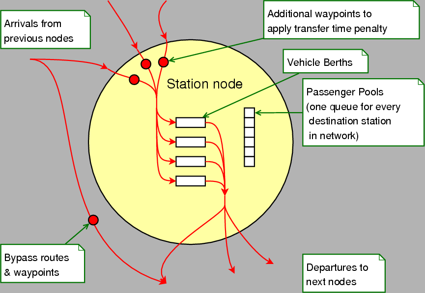
Each neighborhood contains one station cell that corresponds to a node in the transit network. As illustrated in Figure 4.4, all passengers transferring through a station are sorted into PassengerPool containers, one for each other station node in the network. While every passenger in a PassengerPool has the same final destination, they might take separate vehicles or even entirely different paths to get there. Additionally stations have a fixed number of vehicle berths that serve to constrain the maximum number of vehicles that can dock simultaneously. Figure 4.4 depicts a conceptual model of what a station node might look like for the purposes of our scenarios.

Station pairs are connected to each other via arcs defined in a connectivity matrix. Each type of vehicle has its own connectivity matrix, so different modes of transit can serve subsets of stations.

Waypoints

Typically, waypoints are sets of coordinates that identify a point in physical space. To make the modeling language a little more realistic, we added ``non-station'' waypoints on arcs between stations. Waypoints allow for the modeling of systems where stations separated by varying distances (albeit in terms of integer units of time). Waypoints also allow passengers and vehicles to have a defined state while en route between stations while only moderately increasing the number of variables added to the optimization problem.

In the context of this project, waypoints act as one-way nodes in the transit network that allow the system to preserve the state of vehicles and passengers while traveling in-between stations. There are no constraints that prevent passengers from transferring between vehicles at the same waypoint, so to prevent passengers from train-hopping or plane-hopping en route, we apply an additional constraint that all the passengers and vehicles that enter a waypoint at one timestep must leave it the next timestep.

For some models, we might desire this kind of behavior. We could eliminate these waypoint constraints and allow vehicles to effectively enter a holding pattern at a waypoint just outside of a station. And there have been studies and patents filed to allow vehicles to transfer passengers at speed. In the future we may want to ease those constraints somewhat to allow these other types of behaviors.

Waypoints don't really belong to any parent cell in any meaningful way, since they are an artifact of the separate transportation infrastructure overlay as depicted in Figure 2.6. Other entities in the simulation have little reason to interact with them. We typically attach all waypoints directly to the master city cell since they would typically exist between neighborhoods.

We use waypoints to serve two purposes. While they are primarily used to represent the time and space traversed by vehicles between stations, they can also represent only the time spent waiting at a station. In this mode, they would account for time spent slowing down and docking at a station berth, loading and unloading passengers, and - to some extent - the walking time of passengers between platforms or gates while transferring within the station.

All of the scenarios in this work employ at least one waypoint between stations in order to provide a time savings advantage to a vehicle bypassing a station. We use this measure to study the possible performance benefits of having offline stations, which is a feature necessary for rail service with express routing or almost any PRT-like transit proposal.

Vehicles

The vehicles in the various transit fleets traverse the network picking up passengers from stations and dropping them off at the next station. A completely separate transit layer represents each type of vehicle, with their own connectivity matrix that defines the segments and waypoints that each set of vehicles can traverse. The schedule optimizer only cares about two properties for each vehicle type: the maximum passenger capacity and the cost per segment traversed.

TransitTokens

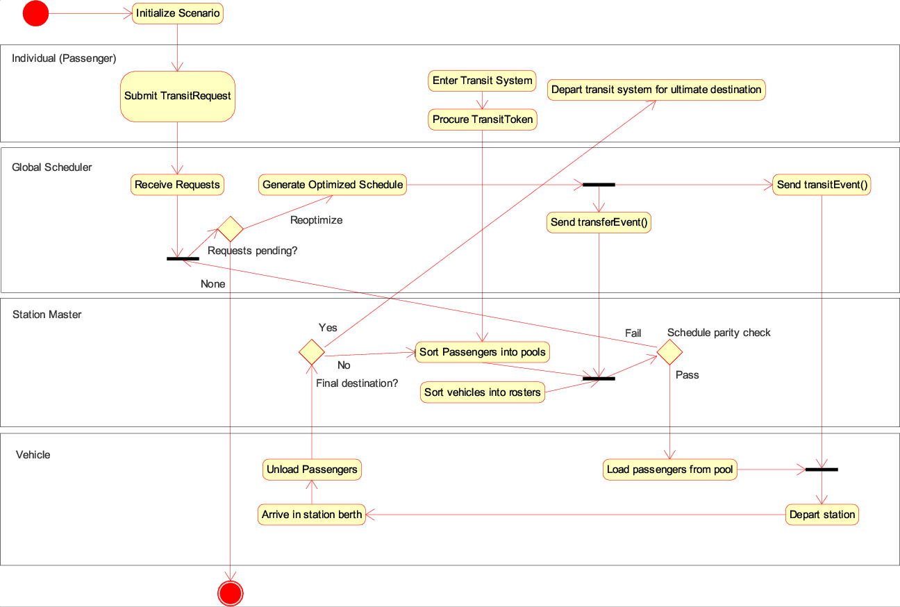
The station master issues TransitTokens to identify passengers and cargo within the transit system, using them to store a customer's final destination. TransitTokens provide a handle used to sort passengers at each transfer station. Additionally, they log the path taken and timestamps for each passenger, so they come in handy for collecting data on transit times and wait times during post processing analysis.

Figure 4.5: Transit Simulation Activity Diagram