Concept Requirements

This section describes the pathway from high-level goals to specific use-cases for the transit system, the mass transit optimization goals, fleet schedule optimization objectives, and transit use cases.

Mass Transit Optimization Goals

This simulation constructs a simple transit network with passengers traveling from source nodes to destination nodes. The scheduler attempts to provide an optimal or quasi-optimal schedule of transit fleet vehicles with various capacities, operating costs, and nodes serviced that will transfer the passengers to their final destination. Through parametric analysis of different demand loading and network topologies, we hope to define some characteristics of urban areas that enable the system to meet the opposing passenger demand and vehicle utilization objectives efficiently.

Fleet Schedule Optimization Objectives

The objective function of the transit vehicle schedule optimization is a weighted composite of the number of passengers served, the time they are delivered, and a flat cost incurred per vehicle leg traveled. The weight on each objective typically puts them on different orders of magnitude, such that a secondary objective should not be considered a factor until the primary objective reaches an optimal configuration.

The relative weighting of objectives is arranged as follows:

$Objective\;1\gg Objective\;2\gg Objective\;3\gg Objective\;4$

Objective 1: Maximize the number of passengers delivered to their final destinations. All passengers are currently weighted equally, which means during instances where the system is operating beyond capacity, the optimizer will favor passengers who are close to their destinations. There is currently no zone tracking to ensure that passengers traveling long distances can ``pay more'' to compensate for the higher transit cost. The objective function also provides no reward for moving passengers partway, so a feasible solution will either move a passenger all the way to their destination node or not at all.

Objective 2: Minimize the amount of time the passengers spend in the transit system. This is accomplished by adding a linear bonus term to the objective function that rewards the system for delivering passengers to their destinations at earlier times. These terms push the schedule ``left'' towards earlier arrival times. Otherwise the system would allow people to wait unnecessarily during the time window under consideration.

Objective 3: An optional objective to minimize deviation from a desired fleet size can be activated. We could simply minimize the number of vehicles in use, but we'd have to find some way to balance this with the passenger service objectives. Plus, most service operators have a fixed number of vehicles and drivers to employ. The optimizer could take advantage of extra vehicles to improve passenger service quality, as well as make recommendations at to when the operator might want to rent additional vehicles and drivers temporarily to meet demand.

Objective 4: Minimize the operating cost of moving vehicles. This is currently expressed by a simple flat cost incurred by each segment a vehicle travels. Each size vehicle could have a different cost per segment traversed, such that a vehicle with a higher capacity would presumably have a greater cost per time unit. Currently the system deducts no cost for vehicles idling at stations, but we could insert this term easily enough if called for.

The objective function is subject to the following constraints:

Conservation of passengers and vehicles moving between nodes. Passengers and vehicles should be neither created or destroyed during the course of the schedule. The MIP schedule optimization follows a classic inventory management problem formulation.

Passenger movement between nodes is constrained by the capacity provided by vehicle movements between nodes. Passengers can only move around in the network when carried by vehicles. The optimization problem currently allows passengers to wait and transfer freely between vehicles at station nodes.

Vehicle movement about the transit network is constrained by several factors:

• Connectivity matrices allow certain types of vehicles to travel only between connected nodes. This allows us to connect nodes together with one or more modes of transit. For example, a certain subset of nodes could be served by a rail system, while the rest of the nodes would only be accessible via bus service. The connectivity matrix provides enough flexibility to model a transit system as a collection of directed graphs, so stations could be connected by one way or bi-directional links.
• Station and waypoint capacity constraints could prevent too many vehicles from visiting the same station or route simultaneously.
• A hard maximum fleet size might prevent some unrealistic solutions.

We could add some arbitrary constraints somewhat easily. For instance, we could limit the maximum number of vehicles on a group of segments or waypoints that have been grouped together to block each other on a constrained resource, such a bottle-necked intersection. This concept is discussed in more detail in Section .

This optimization make no attempt to handle meeting passenger required times of arrival (RTA). It only optimizes based on the reported time passengers first become available to depart. Oftentimes people would want to arrive at their destination just before the fixed start of their work day, or at an airport in time to catch a flight. Because this optimizer uses an inventory management approach, adding this information would result in an exponential increase in decision variables. This added complexity would make the schedule take much longer to generate. Combined with the fact that several of the passengers would not even make use of this functionality (such as the ones who are leaving work and just want to get to their destination as soon as possible), the schedule optimizer declines to consider this constraint.

To add an RTA handling feature, an algorithm external to this schedule optimizer would need to provide a rough estimate of the required time of departure (RTD) necessary to meet a passenger's RTA, and submit a transit request with that RTD into the optimization. If the itinerary provided back to the passenger falls behind (or too far ahead) of their desired arrival time, the algorithm could redact the transit request and try again with a slightly adjusted RTD. A few cycles of this incremental optimization on a much simpler schedule optimizer for the subset of passengers who actually need it should provide an acceptable solution more quickly than if the scheduling problem was reformulated to include variables and objectives to take everyone's RTAs into account.

Transit Use Case Diagram

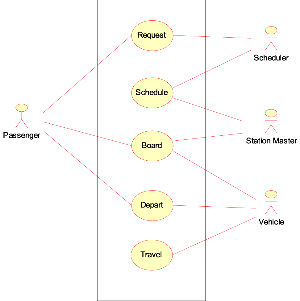
A passenger begins by submitting a transit request for sometime in the future to the global scheduler. The scheduler collects requests and generates an optimized vehicle schedule that separates passengers into several pools based on their current and final destination node. When the time comes to act upon the schedule, a station master at each station loads waiting passengers into the proper vehicle, and then sends the vehicles on their way towards their next destination. When the passenger reaches their final destination, they exit the transit system.

Figure 4.1: Transit use case diagram

For simplicity, this simulation unboards all passengers at each station so the station master can re-sort them into their next/final destination pools. Another logistics layer could be implemented to provide the convenience of maximizing the number of passengers that could stay aboard their vehicles during stops at transfer stations.