Parametric Analysis

To evaluate different transit paradigms, we'd want to reduce the relationship between system design variables and performance metrics into a series of parametric equations. We could then compare the projected levels of investment necessary for infrastructure and operations under competing transit paradigms to meet similar performance goals.

Design of Experiments

We set up a factorial experiment to determine the impact of several design factors. By individually varying each independent variable and observing its effects on our performance metrics, we can establish correlations between our design inputs and system outputs across a variety of conditions.

The scenario generation script populates a full factorial directory tree of 144 scenarios using the following input values for each parameter of interest:

Topology type: [1D rail, 1D rail w/ express service, 2D hexagon, 2D hexagon w/ express service] All topologies consist of 7 station nodes. The ``express'' routes indicate that vehicles may bypass offline stations to gain a 1 time segment advantage over stopping.

Load [4, 64, 128, 256] Passenger demand per station. The total number of passengers on the network would work out to $\frac{6}{7} {Load}$, since $\frac{1}{7}$ of the employees would live in the same neighborhood where they worked.

Vehicle berths per station [2,4,8] Maximum vehicles that can visit and transfer passengers in a station simultaneously per time step. 2 could represent a typical rail station with cars running on 1-way tracks. 4 might represent a rail station with two tracks where cars at the platform could depart in either direction. Finally, 8 could represent a station with many individual, independent berths, such as a bus transfer station.

Vehicle capacity [16, 64, 128] Maximum number of passengers that can ride in each vehicle

A post processing script collects the following output metrics (condensed forms of the histogram data in Section 5.5) and summarizes them into rows on a spreadsheet:

• Total number of passengers handled
• Mean passenger transit time
• Mean passenger departure delay from time available to depart
• Mean passenger number of stops / transfers experienced
• Total number of each vehicle type utilized
• Total number of vehicle segments traveled, to give an estimate of operating costs
• Mean vehicle capacity utilization percentage, to summarize how 'full' the vehicles are running during each segment they travel. This metric gives some indication as to the system's operating efficiency)

Each row of input and output data on the summary spreadsheet represents a different demand level and transit network configuration. We can then use this spreadsheet to generate several families of plots that characterize the performance impact of a range of design input variables. Each of these plots include data regression curves useful for highlighting correlations and for creating an approximate parametric model of transit system design. By applying data filters to the spreadsheet, we can quickly create several plots that compare the different major design paradigms.

Comparison of Linear and Express Routing

We can use our factorial analysis to perform a quick comparison of design factors. In this case, we'd like to highlight some of the performance differences between a transit network with sequential routing and one built to accommodate express routes that can bypass intermediate stations.

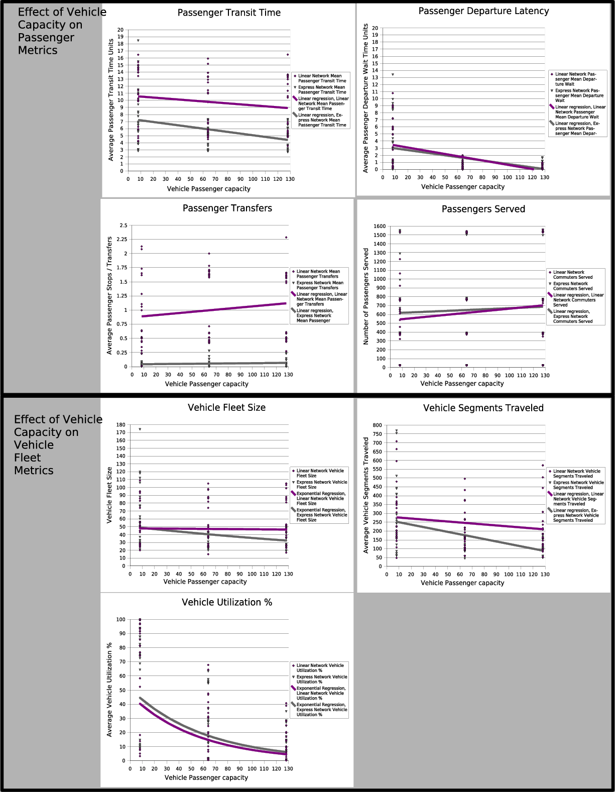
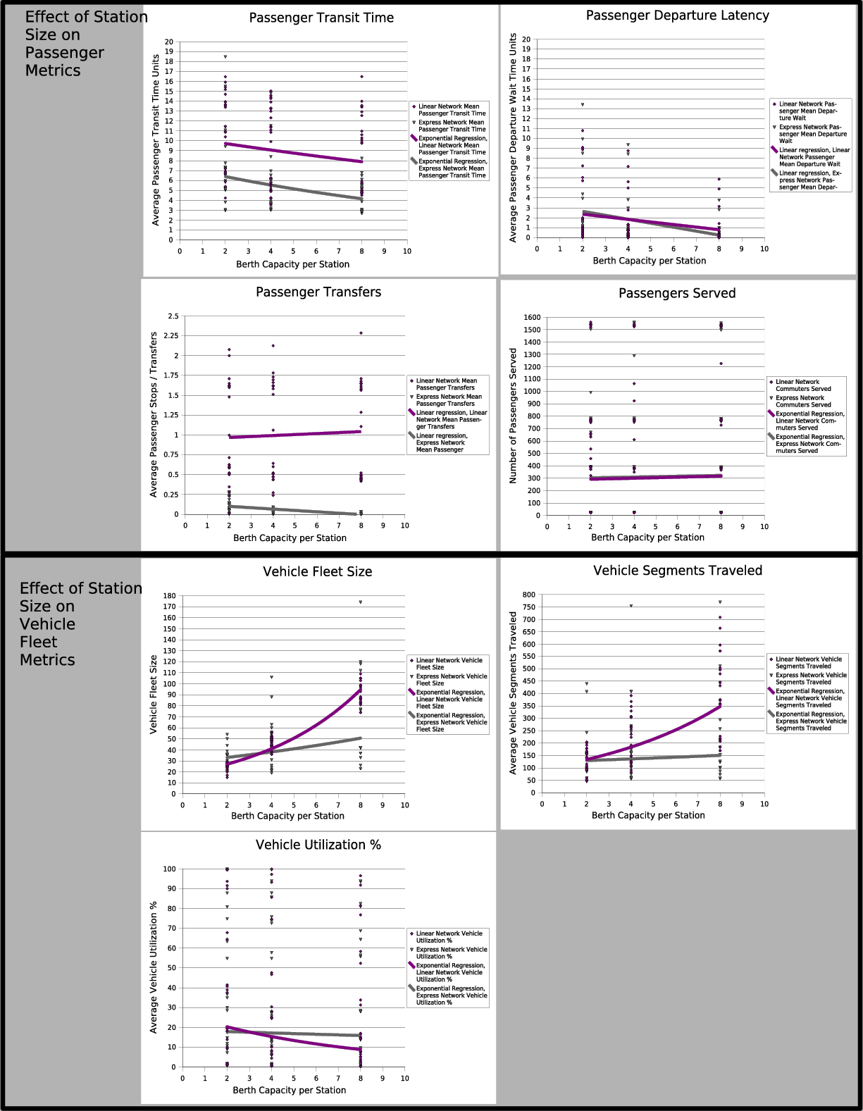
Figures 5.13 and 5.14 plot both the linear sequential routing scenarios and the express routing scenarios on the same set of factorial sensitivity plots for two other design factors (vehicle capacity and station capacity, respectively). A regression line through the data indicates the correlation between the design factor and the performance metric of interest averaged over all of the scenario conditions. A positive or negative slope indicates a correlation, a relatively horizontal regression line suggests that other factors dominate.

The top four charts in each set concern the impact of the design factors to passenger metrics, the bottom three charts affect the vehicle fleet performance.

Figure 5.13: Effect of vehicle size on passenger and fleet performance metrics: a comparison of linear vs. express routing

Figure 5.14: Effect of station size on passenger and fleet performance metrics: a comparison of linear vs. express routing

The charts in Figure 5.13 show that vehicle capacity has little impact on passenger service for our optimized schedules. However, the type of routing used does have a profound impact on the average transit time and number of stops experienced by passengers. Allowing express routing to bypass stations can cut average transit time almost in half, while practically eliminating most stops and transfers.

The number of vehicles necessary to run a schedule and the amount of segments they run is also reduced. The reduction in segments comes about in large part because stops and transfers count as segments. While this may not be an accurate portrayal in terms of mileage saved, this could still represent savings of fuel and vehicle wear-and-tear, as braking and accelerating at a station can be every bit as taxing as cruising at a constant speed for many types of vehicles.

Figure 5.14 tells a similar story, though this time showing that increasing the number of vehicles that can dock at a station simultaneously can get passengers to their destinations more rapidly by easing congestion.

An additional curiosity shows that higher station berthing capacity can result in much a higher fleet size and operating costs in the linear sequential routing case which does not affect the express routing network much. This highlights some of the inefficiency of forcing vehicles to stop at every station along a route, especially when there's extra capacity to handle these stopovers.

This design factor analysis supports notion that, all inputs being equal and subject to our assumptions, an intelligently scheduled mass transit system designed around a larger quantity of smaller vehicles running direct point-to-point routes between offline stations could provide much faster passenger service while meeting and exceeding the fleet operational efficiency of more conventional systems.