Sample Scenarios

The simulation generates histograms plotting the transit system's response to input demand ``pulses''. The demand pulse is currently a one-time uniform random distribution across all source and destination nodes. The simulation generates demand by creating one employer cell in each neighborhood that employs a fixed number of commuters. The employees originate from any station node in the network with a uniform random probability. This arrangement for defining transit demand was chosen to reflect the fact that municipalities often have more control of where and how many jobs are created than where people choose to set up residences.

Scripts produce sets of results for two types of transit topologies meant to represent extremes that would combine to form complete transit network graphs: (1) a simple 1D linear light-rail system, and (2) a 2D hexagonal cluster unit on a triangular grid. We simplify our analysis by limiting the cluster size we consider to only 7 nodes, near the practical limit for computing quasi-optimal solutions to TSP-type problems. We arrange the stations in a simple line, or clustered into a fully-connected star topology with a central hub and six points.

1D Light Rail Transit Network

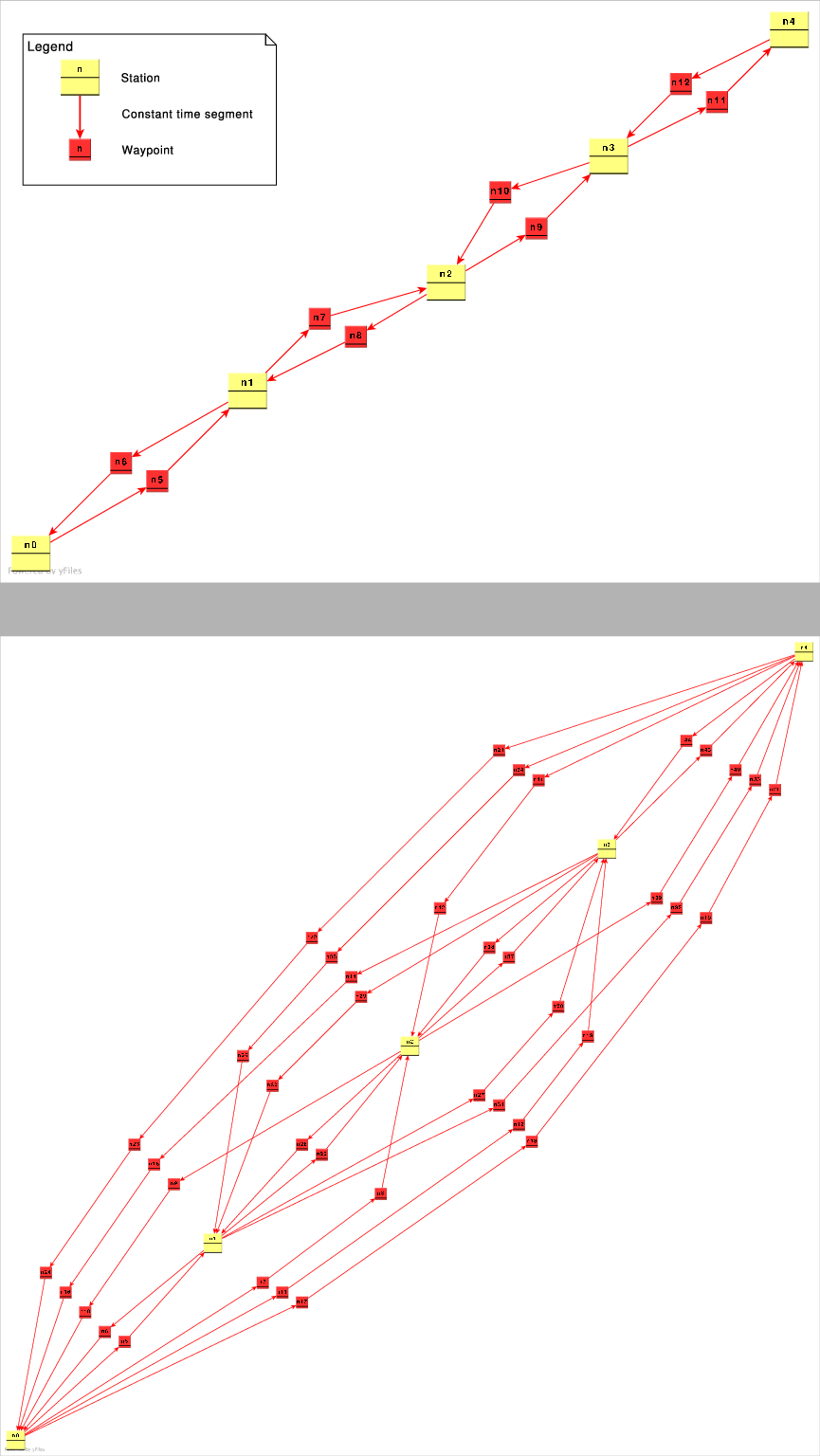
The light rail system has two types of operation: a sequentially-routed ``linear'' rail network where trains must stop at every station, and an ``express'' rail network where stations are off the main line and trains can save time by bypassing stops. Note that the additional routes made available indicate temporal paths and not separate physical paths between stations.

Figure 5.4: 1D Light-Rail System Connecting Four Neighborhoods`
Figure 5.5: 1D Light-Rail System Connecting Four Neighborhoods, but with Local and Express Bypass Routes

2D Hexagonal Network

In order to scale up our schedule optimization to tackle larger, more practical transit networks, we'll have to start by concentrating our efforts on a simple triangular grid organized into hexagonal units. Building upon this basic unit, we could eventually decompose larger problems hierarchically into clusters of hexagonal units and solve them in parallel, as described in Section .

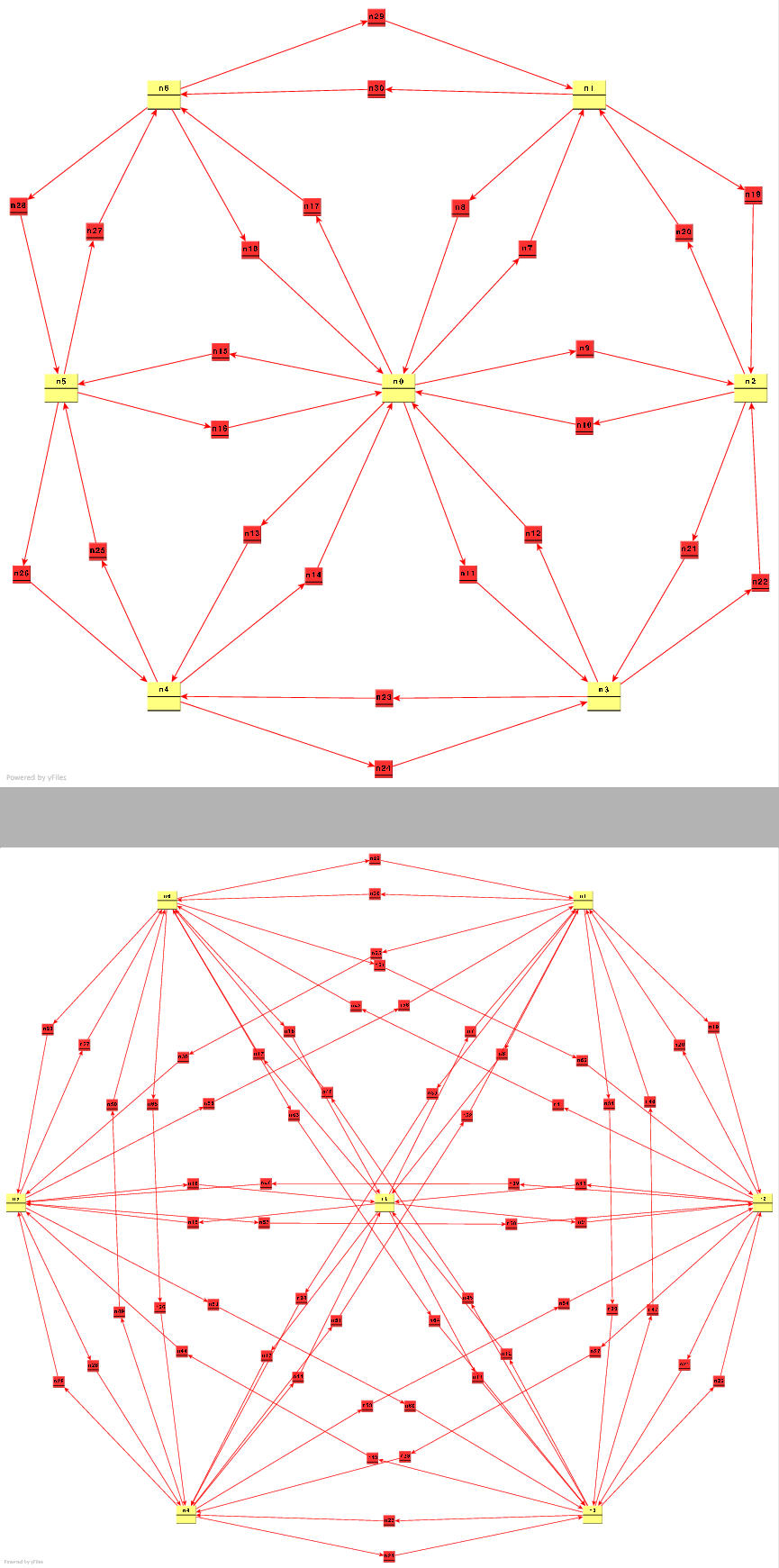
As in the 1D rail scenario, we again distinguish between a sequentially-routed network (depicted by Figure 5.6) where every vehicle must stop for transfers at every station node it passes along its way, and a network with express routes (depicted by Figure 5.6) in which vehicles could bypass stations to save time and berthing space in the stations passed.

Figure 5.6: 2D Hexagonal Cluster
Figure 5.7: 3D Hexagonal Cluster with Express Bypass Routes

Assumptions and Limitations

The simulation currently does not specify all of the initial conditions to the schedule optimizer. In particular, the beginning locations of vehicles are currently left free. This gives the transit systems used in our scenarios an unfair advantage, as vehicles can initially be ``magically'' created anywhere in the network. The total number of vehicles in the fleet is also left unbounded. A more realistic study would consider setting the maximum number of vehicles in the fleet as a design parameter to explore.

To take away some of this advantage, in our scenarios we currently set the final vehicle state to equal the initial vehicle state. This means that each schedule that meets a certain demand pattern is at least repeatable for another run of the exact same demand pattern at the end of its active time interval. It also forces the vehicles to spend some energy returning to their initial state. Since the scheduler considers all vehicles of the same type as interchangeable, this repeatability constraint does not force all vehicles to make complete round-trips. They might operate in rotation with other vehicles of the same type.

As noted in the scenario description at the beginning of Section 5.4, each scenario has a uniform distribution of employers and residents spread out among its nodes, making the problem highly (and uncannily) symmetric. Future studies could easily vary the distribution of demand to model a network with business and residential centers, as noted in Sections and .

Each segment between waypoints and stations represents 2 simulation time units. Typically, the last segment entering a station represents the time penalty for stopping at that station. As seen in the network models, bypassing a station results in a 1 time segment gain. This means that we're assuming that the amount of time a vehicle spends slowing down, stopping, waiting for passenger transfers, and getting back up to speed again is roughly the same amount of time taken to travel between stations at speed. This ratio could be adjusted by adding additional segments to increase the visit penalty at stations, or to increase the travel time between stations. For these scenarios we sill stick to a ratio of $1:1$, which seems reasonable for several forms of transit.

We impose a maximum number of time units allowed by a schedule. Having more time units translates to a higher possible capacity over that time. On the 1D linear rail networks, we limit schedules to 18 time segments, which works out to 1.5 times the diameter of the sequential network ($6*2$ segments between the 7 stations). On the 2D hexagonal networks, we chose a limit of 12 time segments, which works out to 3 times the diameter of the sequential network ($2*2$ segments between an outer station to any other outer station).

Due to the high computing time required to exhaustively search the entire schedule optimization solution space, we impose a time limit on the wall clock time that the computer is allowed to spend finding a solution. When this time limit is reached, the MIP solver will simply return the current best sub-optimal solution it has found. This sub-optimal solution will typically fall close to the final optimal solution, so we could argue that the diminishing improvements to the schedule would not be worth the additional calculation time. In a real transit network this timeout would prevent vehicles from idling while waiting for further instructions from the global scheduler. While this tradeoff may be acceptable for practical purposes, this optimizer timeout defeats the repeatability of our simulation for academic purposes. The CPU would stop computation at a nondeterministic point in the MIP optimization and could return different schedules depending on the speed of the CPU or even on how much time was allocated to other processes in the background. This is a limitation of the LP_Solve software's wall-clock-based timeout feature and could be fixed in the future by adding a deterministic timeout function that returns a sub-optimal result after a fixed number of solver iterations.