Future Work

Chapters 4 and 5 present work that is simply a first step in the development of a comprehensive platform for arcology simulation and optimization. Short-term opportunities for future work could focus on constructing additional studies for factorial analysis, and completing some missing usability features. Long-term development pivots on a major refactor of the schedule generation and interfaces to the simulation that would add detailed modeling features and increase the scalability of the transit network to useful dimensions. In more detail, specific opportunities for future work are as follows:

1. Additional Design Factors. We could easily take the opportunity to design new groups of experiments for factorial analysis on additional design parameters.

1.1. Spatial Load Distribution. Rather than use a uniform random distribution of residences commuting to equal size employment centers scattered throughout the network, we could introduce ramp distributions that would give us separate employment and residence core sectors. We'd expect this asymmetry to reflect current city layouts, and reduce our vehicle utilization as empty vehicles must backfill those departing from residential stations.

Furthermore, we could also make use of job codes and skill codes to model different distributions of employee or employer types throughout a population. For example, if the skill codes were to correlate to residents' socioeconomic status, we could set up a model to study the impact of efforts to integrate rich and poor neighborhoods.

1.2. Temporal Load Distribution Passengers seldom appear at all source stations at exactly the same time. We could vary the shape of the demand input pulse to gradually inject passengers into stations over time.

1.3. Timeliness of Input Data. The amount of time in advance that a passenger submits a transit request to the global optimizer could affect how well the system can have a vehicle ready to pick that passenger up at their requested departure time. In the worst case scenario, the system does not find out about the passenger until the last moment, when they enter the station and buy a TransitToken to a specific destination. The more advance notice the global scheduler has, the better it can budget vehicles to reduce passenger wait times.

1.4. Multiple Vehicle Sizes. The simulation and optimization formulation are capable of handling multiple vehicle types, so it can provide solutions using a mixed fleet of small and large vehicles. The vehicles might even have different connectivity matrices. We'd need to adjust the factorial design generation and simulation monitor taps to allow data collection on multiple vehicle types so we can investigate what pairings of relative vehicles sizes work well.

2. Usability Enhancements. These additional user interface features would aid debugging and assist in further development.

2.1. Simulation Visualization Tool. We need a way to animate schedule results to help verify the simulation visually. Currently the only way to piece together passenger and vehicle movements is to compare schedule spreadsheets at each time step and to trace individual travel histories at the end of the simulation.

2.2. Scenario Editor GUI. In concert with developing an output visualization tool, we'd also want a visual tool for manipulating input data. We currently define scenarios programmatically.

2.3. LiveCD Packaging. The build and execution environment for this project is moderately involved with respect to software dependencies. To this end, we could create a bootable LiveCD based on KNOPPIX that could turn any compatible PC into a full development and compute node [29].

3. Feature Completion. The core simulation engine and modeling language lacks some important features that prevent this project from achieving nominal functionality and modeling realism. Implementing the following features would go a long way towards applying this simulation to practical problems.

3.1. Schedule Optimization State Initialization. The simulation currently has limited support for initializing the state of a schedule optimization. As discussed in Section 5.4.3, we currently do not take the trouble to initialize the current positions of vehicles or existing passengers in the transit network. Adding this internal transfer of initial data constraints would allow us to update and re-optimize a continuously evolving scenario, allowing us to achieve a rolling time horizon type of schedule optimization.

Without this enhancement, we can only run one schedule optimization per scenario with the assumption that the vehicles magically appear where they need to start, and no new information can affect the execution of the schedule once it begins to run.

3.2. Monte Carlo Analysis. We currently use a random seed to provide some entropy in our simulations and create randomized distributions for some input parameters. This means that to properly conduct an analysis, we'd want to run a scenario at least 20 times each with a varying random seed, and perform statistical data reduction on the observed output metrics.

3.3. Constraint Pooling. The system lacks a way to apply capacity constraints to groups of nodes or links, indicating that they share and block on the same physical resource. This would allow multiple routes to share common bottlenecks.

Figure 6.1: Constraint Pooling

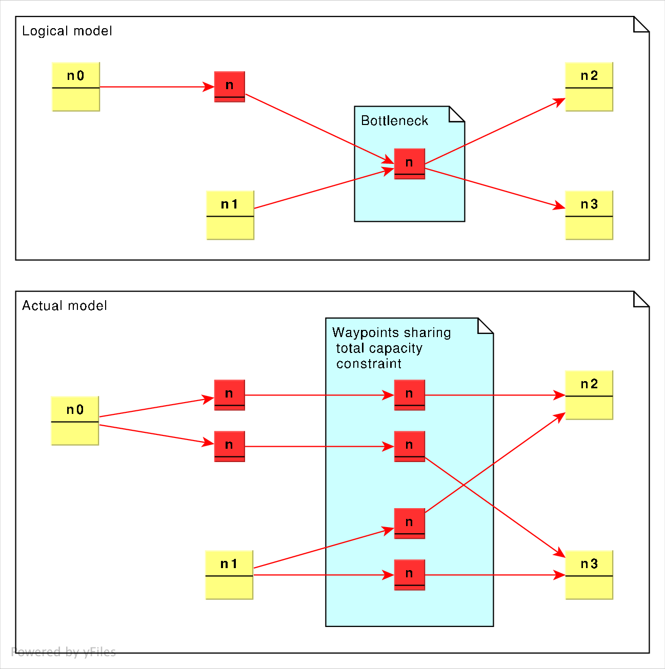
Without the ability to apply a single constraint to a group of nodes, each route linking pairs of nodes would either unintentionally add more capacity between station nodes, or would not allow one route to make full use of the unused capacity of other available routes sharing passage through an intended bottleneck.

3.4. Proper Handling of Long Distance Passengers. The objective function is weighted such that the number of passengers served (objective 1) takes priority over minimizing the number of segments traveled by all vehicles (objective 4). In turn, objective 2 results in ``compression'' of the schedule to the left, in order to complete the schedule as early as possible. The compression is achieved by rewarding the system for sending passengers to their destinations at earlier times during the interval under consideration.

If optimization objectives 1 and 4 were of the same magnitude, we could better balance the conflicting goals between serving passengers at low-volume stations and keeping vehicles filled with paying passengers. The fleet optimizer could possibly even refuse to provide service to low-volume stations to increase total operating efficiency. However, this may also cause high volume routes to become unprofitable for cases where the cost of a long route exceeds the fixed reward for sending a passenger to their destination.

To remedy this, we'd need a more sophisticated reward system that would increase the fare value for long distance travelers. This would involve establishing another dimension to the set of passenger variables that would help track their starting point in addition to their final destination. However, this could easily increase the $O^{3n}$ complexity of the optimization problem to $O^{4n}$. We could limit the impact of this additional term by grouping starting nodes together, so we'd end up with a zone-based pricing system. This would reduce the number of decision variables introduced into the MIP while still preserving the effect of variable fares.

Since this project's optimization formulation does not implement a zone-based fare system, the reward for objective 1 must always exceed the possible cost minimized in objective 4, such that no passenger will get ignored for being unprofitable. To ensure this condition holds true, the passenger reward constant must always be greater than the cost of running a vehicle the diameter of the network by a comfortable margin. The next section addresses a means by which we could provide zone-based service.

4. Scalability Enhancements. Once we've fully defined the scope of the schedule optimizer, we can begin looking for ways to improve its performance. The following measures will allow us to harness the power of parallel processing to tackle larger problems in less time.

4.1. Hierarchical Optimization. The current scheduler has problems finding solutions for more than 8 to 10 station nodes. One way to increase the scalability of our schedule optimizer would involve breaking up the problem hierarchically into smaller sets which we can solve in parallel. The structure of our Arcology model already supports this kind of organization, so we would only have to find a way to map the stations and segments of the transit network into this hierarchy.

This scheme would work by grouping all of the stations into well interconnected clusters of no more than a handful of stations each. We'd need to choose an optimal cluster size that we could solve relatively quickly. E. Christian's HCPPT system employs a similar arrangement that optimizes across hexagonal clusters of 7 regions.[13] In our scheme, each cluster of stations will again be grouped into hexagonal super clusters. Splitting the problem space into this self-similar, recursive hierarchy of cell clusters ensures that we apply TSP style optimizations to no more than a handful of nodes at a time to keep computational requirements within reason.

Optimization will start from the highest level first, and will determine how many vehicles would need to be exchanged between regional clusters. These regional fleet schedule numbers will feed down as boundary conditions to the next lower level in the hierarchy. Now we can solve each sub cluster in parallel, each of them reading the regional schedule in as constraints for their own local schedule optimization. In turn, these sub clusters would recursively split into smaller sub-sub clusters until the schedules they produce finally route vehicles directly between individual stations. This optimization scheme allows us to reduce the computation time for a network of $n$ nodes from $O^{3n}$ to $\frac{n}{m}*O^{3m}$, where the constant $m$ represents the cluster size and $\frac{n}{m}$ is approximately the number of levels in the hierarchy. The cells at each level could be solved in parallel provided enough CPU resources were made available.

The catch is that the higher level regional scheduling takes precedence over local scheduling. On the bright side, this also nicely takes care of the zoned transit problem discussed in the previous Section . However, we must use caution while rationing out station and vehicle capacity constraints so the higher level schedules leave some capacity to serve local passengers.

One possible self-similar recursive structure we could use to partition large problems is a modified heptree. Originally introduced by Bell in 1989 [7], it has several useful properties for our purposes. First of all, the cluster size $m=7$ is near the maximum limit of conveniently computable TSPs. The hexagonal form has also been chosen for other mass transit optimization works, such as for local pick-up and delivery in Cristi$\acute{a}$n Cort$\acute{e}$s' proposed HCPPT network [13]. Here, each vertex serves as a node. Each level of the hierarchy has a slightly different radial orientation relative to its immediate children, but this does not present a major problem for our purposes (compared to others who have considered using this structure). [28] We would overlay the entire structure top of a triangular grid created with waypoints, the segments of the grid representing possible transit network links. The distinguishing feature of our structure from conventional heptrees is the additional padding space that we can place between clusters, as depicted by the white space in Figures 6.2-b and 6.2-c.

Figure 6.2: Recursive self-similar 2D space-filling Heptree Hierarchy

Counter-clockwise from top left:

(a).

Cluster of 7 station nodes

(b).

2 level hierarchy of 49 station nodes

(c).

3 level hierarchy of 343 station nodes

This structure has some interesting properties that gives it some flexibility. First of all, not all nodes or sub clusters in the hierarchy need be fully populated or connected, so we can remove elements until we have a reasonable approximation of local conditions due to geographical or other constraints imposed on development.

Furthermore, the padding between distance between clusters on the same level of the hierarchy is configurable. We have our clusters separated by 1 segment, but this could be uniformly be increased to provide more open space separating the clusters. The padded area might make good undeveloped area to turn into parks, easements, and greenways. If all transit links crossing these padding areas were constrained to bridges or tunnels, pedestrians and migratory wildlife would have free passage across the land via virtually unbroken natural woodlands.

Clusters might be connected to each other in some combination of two different paradigms. We might enforce hub-and-spoke connectivity, where clusters are only joined by high capacity arterial lines (represented by the bold lines in Figure 6.2) linking their central hub nodes together. Alternatively, clusters might also be joined by the fine individual segments of the triangular mesh linking their adjacent sub-clusters together. Traffic could filter through that lattice in a highly distributed fashion.

Whether the arborized or reticulated mode of connectivity dominates likely depends on the scale. Clusters at a neighborhood level would likely follow the hub-and-spoke model, channeling all traffic to a central mass transit station or a highway on-ramp, limiting through traffic through more restricted access. At a regional level, we'd want a more fully connected lattice so we could travel directly toward our destination without going out of our way to transfer at downtown hub stations. However, at the intraurban level, we'd again expect to see more arborization again as we'd funnel our access through consolidated airports or central high speed rail stations.

4.2. Optimization Heuristics. Finally, after we've ensured that we've achieved all of our desired functionality, we can look into other ways of optimizing computational time. The fleet schedule optimizer's work grows exponentially with the number of nodes, so LP_solve reached a scalability limit with merely 8-10 fully-connected stations. Beyond that, it takes more than 30 minutes for a 1.87Ghz AMD K7 PC to find any feasible suboptimal solution. Trying CPLEX instead of LP_solve might help here, especially if CPLEX can do better preprocessing to eliminate variables.

Breaking the problem down into smaller, more manageable chunks would give us our largest performance boost, but there are still other ways we could trim decision variables out of the equation. By strategically pruning MIP branches that provide little performance benefits in comparison to the original algorithms, we could reduce the number of suboptimal dead ends that the optimization engine wastes time exploring. We would want to continue to optimize the algorithms until the scheduler is responsive enough to complete a recovery plan before the next time step. This would allow the system to react to service disruptions as soon as practicable.

Additionally, many of the decision variables in the formulation are zeros. If we can identify linked pools of variables that are consistently zero, we can prune them from the formulation completely. While a MIP solver's presolver should already do a good job of eliminating many of these extra rows from the problem, we could possibly cut down a significant fraction of its work and memory footprint.

5. New Modeling Features.

5.1. Holding Pattern Waypoints. Waypoints currently exist to give vehicles and passengers a state of existence while in transit in between stations. In order to prevent passengers and vehicles from mixing while they are grouped in the same waypoint bins, however, we must apply some additional constraints to effectively prevent mid air passenger transfers between vehicles. The constraints stipulate that all vehicles and passengers that enter a waypoint during one time step must continue on to the next waypoint in lockstep. All waypoints are constructed as part of one-way routes, so there is no possibility of capturing passengers en passant.

To be fair, there have been proposals for improving transit efficiency by docking moving vehicles together and transferring passengers while in motion. [9] So it's comforting to know that we could model some of those scenarios by relaxing constraints.

However, sometimes we do want to allow vehicles to wait or enter ``holding patterns'' at waypoints, so they can create a buffer into another constrained resource, such as an airport runway or gate. This provides additional storage holding capacity outside of the station which can be put to use to increase network capacity. Mostly these buffers are used to help deal with uncertainty. Since our scenario schedules are deterministic, unperturbed by mechanical failures or passengers and vehicles turning up later than they're expected, we would gain little by allowing vehicles to hold at waypoints. Each holding waypoint would also double the number of decision variables needed to hold the new possible states as vehicles can decide to hold or proceed with their passenger load. Due to these factors, waypoint holds have been skipped at this time, but could add a useful modeling element later.

5.2. Continuous Time Model Definition. Currently a model must be expressed in synchronous integer time steps in order to work with the optimization formulation. We'd find it quite useful to define a modeling language that allows us to construct the model with constraints and distances expressed in terms of continuous time.

We could then use algorithms to convert the continuous model into an integer time step model. This would likely introduce a lot of rounding and aliasing artifacts, the effects of which must be quantified and tracked. However, we'd gain the ability to run the same model at varying temporal granularity. This would allow us to study and set an optimal time step length that keeps these errors in check, instead of wasting time manually shoehorning physical models into approximate models using integer time quanta. This flexibility would greatly help address some of the issues introduced by the synchronous integer time step paradigm by allowing us to analyze the same scenario with different timing parameters, observe, and minimize the aliasing artifacts.

A continuous time modeling language would define capacity constraints in fractional units, such as vehicles per unit time. The ability to adjust the resolution of time steps allows us to detailed models with fine-grained time steps over an interval of interest, and solve coarse models much faster. The constraint values must scale with the time step length, such that double the capacity could pass through a constrained node in double the time.

Best of all, this continuous time model might allow us to more easily link together schedules of transit systems that have different paces of operation over different time intervals. For example, high frequency bus and rail transit could effectively serve low frequency but higher capacity airplanes or ships at port. This concept provides a nice segue into the next section, discussing the challenge of coordinating schedules across modes of transit commanded by different fleet operators. Instead of a single organization asserting full sovereignty over all vehicles in the system, we'd want to provide a way to tie together disparate fleets by allowing operators to cooperate on forming a mutually optimal schedule.

5.3. Multiple Operator Collaboration. A global optimizer that could include multiple independent operator goals and scheduling constraints certainly isn't out of the realm of possibility. A central authority would maintain the global schedule formulation, and might allow participating members to add their own sets of constraint statements, or even weighted objective functions. This would allow individual fleet operators to synchronize schedules or even share coverage and balance loads with other fleets. Additionally, they can insert crew and maintenance schedules into the global scheduler to allow them to pick up and drop off drivers, pilots, and other staff at certain locations, or make sure that their vehicles end up in a certain maintenance bays every so often for refueling and service.

These inputs into the optimization problem can take the form of additional constraints. Constraints tend to help reduce the number of branch and bound paths that the optimizer needs to search to converge on a solution. As long as the solution remains feasible, expressing these constraints would be the job of the separate transit fleet organizations. The challenge comes in defining the abstract protocols needed to express these constraints, as they not only would require extensive knowledge of how the global optimization problem is formulated and solved, but should also not be too explicit as to preclude changes and updates to the underlying formulation. It is undesirable to have this information format coupled too closely to the formulation, such as down to the level of variable naming conventions or specific MIP techniques for enforcing certain condition. This lock-in would make it more difficult to change and upgrade the optimization engine in the future. We wouldn't want to force every operator to radically change their code at the simultaneously every time system needs an incremental upgrade. We also wouldn't want a systems upgrade project to fail because of one or two late development efforts. We want enough abstraction built in so that participants might make changes at their own pace to take advantage of newly introduced scheduling and optimization features. The protocol specifying their constraints needs the ability to ``compile'' itself from an abstract to an explicit form so it can translate into both older and new versions of the optimization formulation.

Unfortunately, the design and specification of an abstraction language lies beyond the scope of this work, but we'll outline some of its major requirements. Such a language might allow the businesses to express what additional criteria a generic schedule optimizer must meet, without ``cheating'' and taking advantage of direct and specific knowledge of the optimization formulation and of its variables. A sophisticated abstraction language processor would have to take the expression and transform them into equations that relate particular variables to each other and existing variables in the global problem formulation. This processor would be nontrivial to implement without a lot of prior experience, and even still could give way to unexpected errors and behaviors.

A simple, minimalist collaborative scheduler would allow input of operator-specific crew and vehicle maintenance schedule statements in the form of: ``these vehicles must go off line at this particular station at a particular time step.'' This would imply that the operators determine their maintenance schedules separate from the globally optimized schedule, and then insert service stops as fixed constraints. These constraint inputs would be similar to the scheduling interface used to import legacy systems operating on fixed timetables. The end result of would not be as optimal compared to a system in which the global scheduler could directly search for solutions that also fulfilled operator schedule requirements, but at least they would start closer to an optimal solution. The iterations could proceed as follows:

1. The transit network operator provides the number and current locations of available vehicles at the beginning of the day
2. The global optimizer takes the customer demands and those initial conditions, and furnishes the schedule desired of that transit system.
3. The operators manually (or semi-heuristically) tweak the schedule to ensure that particular vehicles end up in nearby maintenance bays when they're due. These get fed back into the global optimization as constraints.
4. The global optimizer finds another solution taking these new constraints into account, filling in any gaps created in the schedule and hopefully not straying too far from the original optimal objective function result.

This would let us converge on a schedule somewhat near the optimal one that takes maintenance factors into account without tying down the program formulation to a particular implementation of the optimizer. A more sophisticated collaborative optimization scheme with a more expressive abstraction language would be able to tell the global scheduler where its maintenance bays were located and how often each vehicle needs to visit them, allowing the global optimizer to include fleet maintenance requirements after a single pass of schedule generation.

We'd still need to exercise some discipline to keep the system stable. In a transit system run by a single operator, the entire problem formulated by one party and all the input data provided by passenger requests and vehicle locations add constraints in a consistent manner - the worst possible outcome caused by injecting faulty data might be infeasibility. However, by allowing third parties deeper control of objective functions and constraint statements, we're opening up the system to a host of potential pitfalls and vulnerabilities:

• Malformed or even malicious statements could make the problem intractable. There may be ways to identify some offending statements and automatically detect and flag them to somehow alert or even filter them out of the calculations. However, the latter approach could just as well create unpredictable results by orphaning variables (and thus leaving them unbounded).

• We'd need ownership and permissions on variables to separate the MIP components provided by different parties. This would ensure that operators don't introduce constraints that could penalize their competitors. This could be accomplished by prefixing variable names with namespaces and restricting access to allowed or ``safe'' variables.

• Operators could attempt to maliciously game the system by reserving excess capacity for themselves to lock out their competitors. This would be more difficult to do, since the global optimizer would balance the passenger load across all fleets.

• Many companies pride themselves on their own optimization capabilities. We may need a mechanism to protect proprietary information about their business strategies revealed in operator's contributed code. We might allow them to submit ``black box'' modules that manage to interact properly with the rest of the global optimization. An alternative method may be to partition the problem such that they're entirely responsible for optimizing their particular segment of the global calculation, interacting with the rest of the system through a layer of input and output variables.

Hopefully these considerations have helped articulate why the current incarnation of this thesis does not address these issues. At the same time, this highlights some of the exciting possibilities and new market opportunities made available by cooperatively linking disparate fleets into a cohesive end-to-end transit system.

5.4. Dealing with Unforeseen Events. Uncertainty is the antithesis to careful planning. Unfortunately, we live in an uncertain world, and need to make contingency plans for when things go wrong. How would the system deal with unexpected events that crop up during the execution of schedules?

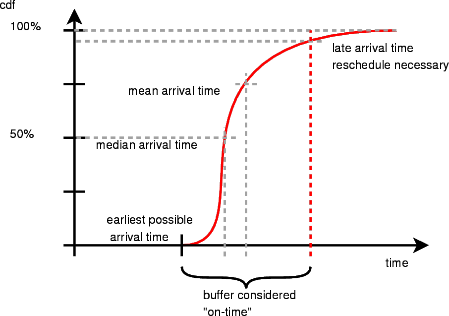
While this thesis project makes no allowance for the possibility of its virtual vehicles getting held up by hail or high water, a practical system should factor in probabilities and fault trees into the schedule formulation. The optimizer might try to minimize is the impact of unfavorable events as an objective. Analysis of historical records can generate probability metrics associated with vehicle failures, route closures, inclement weather prediction, and so forth. A useful way of representing on-time vehicle performance probabilistically is to reconstruct the data from the cumulative distribution function (CDF) associated with the prediction as shown in Figure 6.3. This provides a much more useful picture than a simple mean and standard deviation, since most transit data is skewed towards the right. It's much easier to arrive late rather than early. We could quantize the CDF to reduce MIP formulation complexity, at the cost of adding longer, more conservative wait time buffers between connections. While complete arrival data should be monitored and collected, only vehicles arriving after the late arrival cutoff tail (indicated by the red dashed line) would impact the scheduler and trigger replan.

Figure 6.3: Notional CDF of vehicle arrivals vs. transit time, based on historical records

The trick is to try to minimize the buffer time necessary to keep the schedule stable. Larger buffers would increase the time wasted waiting. We're primarily interested in what time the vast majority of the vehicles will arrive, as well as what hopefully small percentage of late vehicles cause schedule-impacting delays. We have no fixed ``magic percentile'' that would determine how much extra buffer time to schedule to ensure that mostly everyone makes their connections. This tolerance will likely get set arbitrarily at the beginning, as all of these factors contribute to an overall ``schedule volatility'' metric. With the optimizer system, we can recompute new schedules whenever an unexpected event occurs - such as when a vehicle is delayed enough to fall onto the tail end of the CDF and its passengers wind up missing their connections. The optimizer can take that emerging information into account and simply create a new schedule based on these new conditions - in this case it would likely divert other vehicles to pick up the stragglers stranded by the late vehicle. So the risk analysis that determines how aggressively to schedule extra buffers into the system would depend on how much impact a schedule recovery plan would have. Planning in large buffers to reduce the likelihood of major delays means extra wait time for passengers and more idle time for vehicles in order to ensure that the schedule stays stable. The ability to drastically reduce these buffers means the whole system could run at a faster pace. If the cost of recovering from missed connections is low - suppose its a fixed train route that runs every 5 minutes - then the scheduler can comfortably deal with smaller buffers and higher schedule volatility. In the case of an airplane network where flights run between cities maybe once or twice a day, a missed connection would mean putting people up in hotels or chartering additional make-up flights. In this case, increased schedule awareness and dynamic optimization can help by figuring out the total system impact, and balance the cost of holding flights to allow latecomers to make their connections.

In light of this, we would want to introduce some practical optimization goals to the list of transit system performance goals discussed in section 3.1.1. This performance metric would characterize the system's stability in the face of unexpected breakdowns and delays, meaning it would help the scheduler intelligently create and maintain buffers to deal with uncertainty. How to actually formulate and compute this enhancement is beyond the scope of this thesis. The optimizer would likely need to do risk-impact assessments on every combination of missed connection to identify vehicles with critical path routes. But we do wish to ensure that the necessary on-time performance data is collected now, so that future generations of engineers could tackle this issue.